這篇文章記錄我在datacamp學習Supervised Learning with scikit-learn的課程。
什麼是ML?
簡單來說就是給機器資料,讓他有能力去做決定,
而這個決定並不是依賴明確的編碼而產生的過程。
Supervised learning 與 Unsupervised learning 最大的差別在於要不要主動去貼標這件事。
目錄
Classification
EDA(Exploratory data analysis)
- load the dataset
from sklearn import datasets iris = datasets.load_iris() print(iris.keys()) # to see the keys of iris - visual EDA
x = iris.data y = iris.target df = pd.DataFrame(X, columns=iris.feature_names) _ = pd.plotting.scatter_matrix(df, c=y, figsize=[8, 8], s=150, marker="D") - target variable 也就是y值,換句話說就是要預測的值。
- 當features的值是binary時,可以用Seaborn’s countplot來進行EDA。
plt.figure()
# x=feature, hue=y, palette=color of the bar
sns.countplot(x='education', hue='party', data=df, palette='RdBu')
# 0 represent no, 1 represent yes
plt.xticks([0,1], ['No', 'Yes'])
plt.show()  # outcome的x軸會是education,分別是No跟Yes,且在No跟Yes上分別各有兩個bars,indicate出兩parties各有多少人數(party只有民主黨跟共和黨)
classification with KNN
- by using features to predict which parties would the voter vote to
from sklearn.neighbors import KNeighborsClassifier
# Create arrays for the features and the response variable
y = df['party'].values
X = df.drop('party', axis=1).values
# Create a k-NN classifier with 6 neighbors
knn = KNeighborsClassifier(n_neighbors=6)
# Fit the classifier to the data
knn.fit(X,y)
# Predict the labels for the training data X
y_pred = knn.predict(X)
# Predict and print the label for the new data point X_new
new_prediction = knn.predict(X_new)
print("Prediction: {}".format(new_prediction))
Measuring model performance
# Import necessary modules
from sklearn.neighbors import KNeighborsClassifier
from sklearn.model_selection import train_test_split
# Create feature and target arrays
X = digits.data
y = digits.target
# Split into training and test set
X_train, X_test, y_train, y_test = train_test_split(X, y, test_size = 0.2, random_state=42, stratify=y)
# Create a k-NN classifier with 7 neighbors: knn
knn = KNeighborsClassifier(n_neighbors=7)
# Fit the classifier to the training data
knn.fit(X_train, y_train)
# y_pred = knn.predict(X_test)
# Print the accuracy
print(knn.score(X_test, y_test))
Generate plot to see which k is the best
- larger k = smoother decision boundary = less complex model
- larger k = more complex model = can lead to overfitting
- use model complexity to see “overfitting” and “underfitting”
- review: enumerate()
# Setup arrays to store train and test accuracies
neighbors = np.arange(1, 9)
train_accuracy = np.empty(len(neighbors))
test_accuracy = np.empty(len(neighbors))
# Loop over different values of k
for i, k in enumerate(neighbors):
  # Setup a k-NN Classifier with k neighbors: knn
  knn = KNeighborsClassifier(n_neighbors=k)
  # Fit the classifier to the training data
  knn.fit(X_train, y_train)
  # Compute accuracy on the training set
  train_accuracy[i] = knn.score(X_train, y_train)
  # Compute accuracy on the testing set
  test_accuracy[i] = knn.score(X_test, y_test)
# Generate plot
plt.title('k-NN: Varying Number of Neighbors')
plt.plot(neighbors, test_accuracy, label = 'Testing Accuracy')
plt.plot(neighbors, train_accuracy, label = 'Training Accuracy')
plt.legend()
plt.xlabel('Number of Neighbors')
plt.ylabel('Accuracy')
plt.show()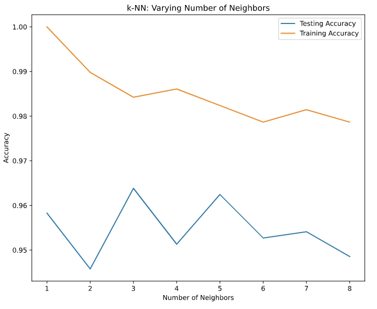
Regression
- regression 的 target value(y) 是連續型的變數,如GDP。
- 以下範例為預測年紀的程式碼
# Import numpy and pandas
import numpy as np
import pandas as pd
# Read the CSV file into a DataFrame: df
df = pd.read_csv('gapminder.csv')
# Create arrays for features and target variable(先僅用出生率做出一個單變數回歸)
X = df['fertility'].values
y = df['life'].values
# Print the dimensions of y and X before reshaping
print("Dimensions of y before reshaping: ", y.shape)
print("Dimensions of X before reshaping: ", X.shape)
# Reshape X and y
y_reshaped = y.reshape(-1,1)  # 假設原先的array有8個elements,reshape(2,4)將變成2rows,4columns的matrix
X_reshaped = X.reshape(-1,1)  # reshape填入-1即代表自動計算(給定另一個的數字的情況下)
# Print the dimensions of y_reshaped and X_reshaped
print("Dimensions of y after reshaping: ", y_reshaped.shape)
print("Dimensions of X after reshaping: ", X_reshaped.shape)
Dimensions of y before reshaping: (139,) Dimensions of X before reshaping: (139,) Dimensions of y after reshaping: (139, 1) Dimensions of X after reshaping: (139, 1)# Import LinearRegression from sklearn.linear_model import LinearRegression # Create the regressor: reg reg = LinearRegression() # Create the prediction space(做出一個等差數列,再轉成matrix,將用來做為測試集) prediction_space = np.linspace(min(X_fertility), max(X_fertility)).reshape(-1,1) # Fit the model to the data reg.fit(X_fertility, y) # Compute predictions over the prediction space: y_pred y_pred = reg.predict(prediction_space) # Print R^2 (regression用R square來看) print(reg.score(X_fertility, y))# Import necessary modules from sklearn.linear_model import LinearRegression from sklearn.metrics import mean_squared_error from sklearn.model_selection import train_test_split # Create training and test sets X_train, X_test, y_train, y_test = train_test_split(X, y, test_size = 0.3, random_state=42) # Create the regressor: reg_all reg_all = LinearRegression() # Fit the regressor to the training data reg_all.fit(X_train, y_train) # Predict on the test data: y_pred y_pred = reg_all.predict(X_test) # Compute and print R^2 and RMSE print("R^2: {}".format(reg_all.score(X_test, y_test))) rmse = np.sqrt(mean_squared_error(y_test, y_pred)) print("Root Mean Squared Error: {}".format(rmse))R^2: 0.838046873142936 Root Mean Squared Error: 3.2476010800377213
Cross-validation
- k folds = k-fold CV
- more folds = more computationally expensive
- 好處是不會剛好在切訓練集時特別衰
# Import the necessary modules
from sklearn.linear_model import LinearRegression
from sklearn.model_selection import cross_val_score
# Create a linear regression object: reg
reg = LinearRegression()
# Compute 5-fold cross-validation scores: cv_scores
cv_scores = cross_val_score(reg, X, y, cv=5)
# Print the 5-fold cross-validation scores
print(cv_scores)
print("Average 5-Fold CV Score: {}".format(np.mean(cv_scores)))
[0.81720569 0.82917058 0.90214134 0.80633989 0.94495637] Average 5-Fold CV Score: 0.8599627722793232
Regularized regression
- goals: penalizing large coefficients by Reqularization because large coefficients can lead to overfitting
- Example 1: ridge regression
- Loss function = OLS loss function + Alpha*sum(coefficients)^2
- (need to select Alpha, like KNN’s k)
- 下例將顯示不同Alpha時獲得不同的score
# Import necessary modules
from sklearn.linear_model import Ridge
from sklearn.model_selection import cross_val_score
# Setup the array of alphas and lists to store scores
alpha_space = np.logspace(-4, 0, 50)
ridge_scores = []
ridge_scores_std = []
# Create a ridge regressor: ridge
ridge = Ridge(normalize=True)  # 原本會是Ridge(alpha=0.1, normalize=True),但這裡不寫alpha留到迴圈寫,為的是顯示出不同Alpha時不同的情況
# Compute scores over range of alphas
for alpha in alpha_space:
  # Specify the alpha value to use: ridge.alpha
  ridge.alpha = alpha
  # Perform 10-fold CV: ridge_cv_scores
  ridge_cv_scores = cross_val_score(ridge, X, y, cv=10)
  # Append the mean of ridge_cv_scores to ridge_scores
  ridge_scores.append(np.mean(ridge_cv_scores))
  # Append the std of ridge_cv_scores to ridge_scores_std
  ridge_scores_std.append(np.std(ridge_cv_scores))
# Display the plot
display_plot(ridge_scores, ridge_scores_std)
- 下面程式碼作為補充
def display_plot(cv_scores, cv_scores_std):
  fig = plt.figure()
  ax = fig.add_subplot(1,1,1)
  ax.plot(alpha_space, cv_scores)
  std_error = cv_scores_std / np.sqrt(10)
  ax.fill_between(alpha_space, cv_scores + std_error, cv_scores - std_error, alpha=0.2)
  ax.set_ylabel('CV Score +/- Std Error')
  ax.set_xlabel('Alpha')
  ax.axhline(np.max(cv_scores), linestyle='--', color='.5')
  ax.set_xlim([alpha_space[0], alpha_space[-1]])
  ax.set_xscale('log')
  plt.show()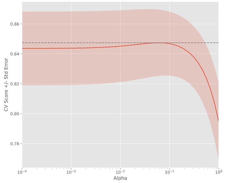
- Example 2: Lasso regression
- Loss function = OLS loss function + Alpha*abs(coefficients)
- can be used to select important features of a dataset
- shrinks the coefficients of less important features to exactly 0
# Import Lasso from sklearn.linear_model import Lasso # Instantiate a lasso regressor: lasso lasso = Lasso(alpha=0.4, normalize=True) # Fit the regressor to the data lasso.fit(X, y) # Compute and print the coefficients lasso_coef = lasso.fit(X, y).coef_ print(lasso_coef) # output: [-0. -0. -0. 0. 0. 0. # -0. -0.07087587] # Plot the coefficients plt.plot(range(len(df_columns)), lasso_coef) plt.xticks(range(len(df_columns)), df_columns.values, rotation=60) plt.margins(0.02) plt.show()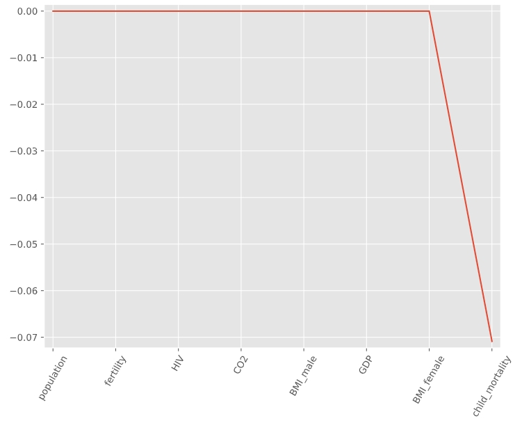 ‘child_mortality’ is the most important feature when predicting life expectancy.
Fine-tuning your model
- Metrics for classification
- KNN
# Import necessary modules from sklearn.metrics import classification_report from sklearn.metrics import confusion_matrix # Create training and test set X_train, X_test, y_train, y_test = train_test_split(X, y, test_size=0.4, random_state=42) # Instantiate a k-NN classifier: knn knn = KNeighborsClassifier(n_neighbors=6) # Fit the classifier to the training data knn.fit(X_train, y_train) # Predict the labels of the test data: y_pred y_pred = knn.predict(X_test) # Generate the confusion matrix and classification report print(confusion_matrix(y_test, y_pred)) print(classification_report(y_test, y_pred)) - Logistic regression (預設的 threshold=0.5,超過0.5判定為1,相反則為0。)
# Import the necessary modules from sklearn.linear_model import LogisticRegression from sklearn.metrics import confusion_matrix, classification_report # Create training and test sets X_train, X_test, y_train, y_test = train_test_split(X, y, test_size = 0.4, random_state=42) # Create the classifier: logreg logreg = LogisticRegression() # Fit the classifier to the training data logreg.fit(X_train, y_train) # Predict the labels of the test set: y_pred y_pred = logreg.predict(X_test) # Compute and print the confusion matrix and classification report print(confusion_matrix(y_test, y_pred)) print(classification_report(y_test, y_pred)) - 製作ROC curve
# Import necessary modules from sklearn.metrics import roc_curve # Compute predicted probabilities: y_pred_prob y_pred_prob = logreg.predict_proba(X_test)[:,1] # Generate ROC curve values: fpr, tpr, thresholds fpr, tpr, thresholds = roc_curve(y_test, y_pred_prob) # Plot ROC curve plt.plot([0, 1], [0, 1], 'k--') plt.plot(fpr, tpr) plt.xlabel('False Positive Rate') plt.ylabel('True Positive Rate') plt.title('ROC Curve') plt.show() - AUROC
# Import necessary modules
from sklearn.metrics import roc_auc_score
from sklearn.model_selection import cross_val_score
# Compute predicted probabilities: y_pred_prob
y_pred_prob = logreg.predict_proba(X_test)[:,1]
# Compute and print AUC score
print("AUC: {}".format(roc_auc_score(y_test, y_pred_prob)))
# Compute cross-validated AUC scores: cv_auc
cv_auc = cross_val_score(logreg, X, y, cv=5, scoring='roc_auc')
# Print list of AUC scores
print("AUC scores computed using 5-fold cross-validation: {}".format(cv_auc))
- KNN
- Hyperparameter tuning(choose the best parameters like alpha and k)
# Import necessary modules from sklearn.linear_model import LogisticRegression from sklearn.model_selection import GridSearchCV # Setup the hyperparameter grid c_space = np.logspace(-5, 8, 15) param_grid = {'C': c_space} # Instantiate a logistic regression classifier: logreg logreg = LogisticRegression() # Instantiate the GridSearchCV object: logreg_cv logreg_cv = GridSearchCV(logreg, param_grid, cv=5) # Fit it to the data logreg_cv.fit(X, y) # Print the tuned parameters and score print("Tuned Logistic Regression Parameters: {}".format(logreg_cv.best_params_)) print("Best score is {}".format(logreg_cv.best_score_)) - Hyperparameter tuning with RandomizedSearchCV(不用再訂範圍了)
# Import necessary modules from scipy.stats import randint from sklearn.tree import DecisionTreeClassifier from sklearn.model_selection import RandomizedSearchCV # Setup the parameters and distributions to sample from: param_dist param_dist = {"max_depth": [3, None], "max_features": randint(1, 9), "min_samples_leaf": randint(1, 9), "criterion": ["gini", "entropy"]} # Instantiate a Decision Tree classifier: tree tree = DecisionTreeClassifier() # Instantiate the RandomizedSearchCV object: tree_cv tree_cv = RandomizedSearchCV(tree, param_dist, cv=5) # Fit it to the data tree_cv.fit(X, y) # Print the tuned parameters and score print("Tuned Decision Tree Parameters: {}".format(tree_cv.best_params_)) print("Best score is {}".format(tree_cv.best_score_)) - Hold-out set for final evaluation(在做K-fold前就先分好training data & testing data,目的是為了更準確衡量model的準確性)
- Classification
# Import necessary modules from sklearn.model_selection import train_test_split from sklearn.linear_model import LogisticRegression from sklearn.model_selection import GridSearchCV # Create the hyperparameter grid c_space = np.logspace(-5, 8, 15) param_grid = {'C': c_space, 'penalty': ['l1', 'l2']} # Instantiate the logistic regression classifier: logreg logreg = LogisticRegression() # Create train and test sets X_train, X_test, y_train, y_test = X_train, X_test, y_train, y_test = train_test_split(X, y, test_size = 0.4, random_state=42) # Instantiate the GridSearchCV object: logreg_cv logreg_cv = GridSearchCV(logreg, param_grid, cv=5) # Fit it to the training data logreg_cv.fit(X_train, y_train) # Print the optimal parameters and best score print("Tuned Logistic Regression Parameter: {}".format(logreg_cv.best_params_)) print("Tuned Logistic Regression Accuracy: {}".format(logreg_cv.best_score_)) - Regression
# Import necessary modules
from sklearn.linear_model import ElasticNet
from sklearn.metrics import mean_squared_error
from sklearn.model_selection import GridSearchCV
from sklearn.model_selection import train_test_split
# Create train and test sets
X_train, X_test, y_train, y_test =  train_test_split(X, y, test_size = 0.4, random_state=42)
# Create the hyperparameter grid
l1_space = np.linspace(0, 1, 30)
param_grid = {'l1_ratio': l1_space}
# Instantiate the ElasticNet regressor: elastic_net
elastic_net = ElasticNet()
# Setup the GridSearchCV object: gm_cv
gm_cv = GridSearchCV(elastic_net, param_grid, cv=5)
# Fit it to the training data
gm_cv.fit(X_train, y_train)
# Predict on the test set and compute metrics
y_pred = gm_cv.predict(X_test)
r2 = gm_cv.score(X_test, y_test)
mse = mean_squared_error(y_test, y_pred)
print("Tuned ElasticNet l1 ratio: {}".format(gm_cv.best_params_))
print("Tuned ElasticNet R squared: {}".format(r2))
print("Tuned ElasticNet MSE: {}".format(mse))
- Classification
Preprocessing and pipelines
- Scikit-learn will not accept categorical features by default
- Create dummy variables!!
- scikit-learn: OneHotEncoder()
- pandas: get_dummies()
# Import pandas
import pandas as pd
# Read 'gapminder.csv' into a DataFrame: df
df = pd.read_csv('gapminder.csv')
# Create dummy variables: df_region
df_region = pd.get_dummies(df)
- Handling missing data
# Convert '?' to NaN df[df == '?'] = np.nan # Drop missing values and print shape of new DataFrame df = df.dropna() # Print shape of new DataFrame print("Shape of DataFrame After Dropping All Rows with Missing Values: {}".format(df.shape)) - impute missing data in a ML pipeline
- make an educated guess about missing values
- example demostrates filling the missing data and apply it into model
# Import necessary modules
from sklearn.preprocessing import Imputer
from sklearn.pipeline import Pipeline
from sklearn.svm import SVC
# Setup the pipeline steps: steps
# The first tuple should consist of the imputation step
# The second should consist of the classifier
steps = [('imputation', Imputer(missing_values='NaN', strategy='most_frequent', axis=0)),
  ('SVM', SVC())]
# Create the pipeline: pipeline
pipeline = Pipeline(steps)
# Create training and test sets
X_train, X_test, y_train, y_test = train_test_split(X, y, test_size=0.3, random_state=42)
# Fit the pipeline to the train set
pipeline.fit(X_train, y_train)
# Predict the labels of the test set
y_pred = pipeline.predict(X_test)
# Compute metrics
print(classification_report(y_test, y_pred))
- Centering and scaling(when your feature has huge difference)
- standardization(minus the mean and divide by std)
- the example below demostrates the difference between w/ and w/o standardization
# Import the necessary modules
from sklearn.preprocessing import StandardScaler
from sklearn.pipeline import Pipeline
# Setup the pipeline steps: steps
steps = [('scaler', StandardScaler()),
  ('knn', KNeighborsClassifier())]
# Create the pipeline: pipeline
pipeline = Pipeline(steps)
# Create train and test sets
X_train, X_test, y_train, y_test = train_test_split(X, y, test_size=0.3, random_state=42)
# Fit the pipeline to the training set: knn_scaled
knn_scaled = pipeline.fit(X_train, y_train)
# Instantiate and fit a k-NN classifier to the unscaled data
knn_unscaled = KNeighborsClassifier().fit(X_train, y_train)
# Compute and print metrics
print('Accuracy with Scaling: {}'.format(knn_scaled.score(X_test, y_test)))
print('Accuracy without Scaling: {}'.format(knn_unscaled.score(X_test, y_test)))
- Pipeline for classification
# Setup the pipeline steps = [('scaler', StandardScaler()), ('SVM', SVC())] pipeline = Pipeline(steps) # Specify the hyperparameter space parameters = {'SVM__C':[1, 10, 100], 'SVM__gamma':[0.1, 0.01]} # Create train and test sets X_train, X_test, y_train, y_test = train_test_split(X, y, test_size=0.2, random_state=21) # Instantiate the GridSearchCV object: cv cv = GridSearchCV(pipeline, param_grid=parameters) # Fit to the training set cv.fit(X_train, y_train) # Predict the labels of the test set: y_pred y_pred = cv.predict(X_test) # Compute and print metrics print("Accuracy: {}".format(cv.score(X_test, y_test))) print(classification_report(y_test, y_pred)) print("Tuned Model Parameters: {}".format(cv.best_params_)) - Pipeline for regression
# Setup the pipeline steps: steps
steps = [('imputation', Imputer(missing_values='NaN', strategy='mean', axis=0)),
       ('scaler', StandardScaler()),
       ('elasticnet', ElasticNet())]
# Create the pipeline: pipeline
pipeline = Pipeline(steps)
# Specify the hyperparameter space
parameters = {'elasticnet__l1_ratio':np.linspace(0,1,30)}
# Create train and test sets
X_train, X_test, y_train, y_test = train_test_split(X, y, test_size=0.4, random_state=42)
# Create the GridSearchCV object: gm_cv
gm_cv = GridSearchCV(pipeline, param_grid=parameters)
# Fit to the training set
gm_cv.fit(X_train, y_train)
# Compute and print the metrics
r2 = gm_cv.score(X_test, y_test)
print("Tuned ElasticNet Alpha: {}".format(gm_cv.best_params_))
print("Tuned ElasticNet R squared: {}".format(r2))